Next: 11.3 Discussion and Exercises Up: 11. Sorting Algorithms Previous: 11.1 Comparison-Based Sorting Contents Index
In this section we study two sorting algorithms that are not
comparison-based. Specialized for sorting small integers, these algorithms
elude the lower-bounds of Theorem 11.5
by using (parts of) the elements in
![]() as indices into an array.
Consider a statement of the form
as indices into an array.
Consider a statement of the form
Suppose we have an input array
![]() consisting of
consisting of
![]() integers, each in
the range
integers, each in
the range
![]() . The counting-sort
algorithm sorts
. The counting-sort
algorithm sorts
![]() using an auxiliary array
using an auxiliary array
![]() of counters. It outputs a sorted version
of
of counters. It outputs a sorted version
of
![]() as an auxiliary array
as an auxiliary array
![]() .
.
The idea behind counting-sort is simple: For each
![]() , count the number of occurrences of
, count the number of occurrences of
![]() in
in
![]() and store this in
and store this in
![]() . Now, after sorting, the output will look like
. Now, after sorting, the output will look like
![]() occurrences of 0, followed by
occurrences of 0, followed by
![]() occurrences of 1, followed by
occurrences of 1, followed by
![]() occurrences of 2,..., followed by
occurrences of 2,..., followed by
![]() occurrences of
occurrences of
![]() .
The code that does this is very slick, and its execution is illustrated in
Figure 11.7:
.
The code that does this is very slick, and its execution is illustrated in
Figure 11.7:
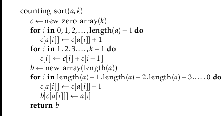
The first
![]() loop in this code sets each counter
loop in this code sets each counter
![]() so that it
counts the number of occurrences of
so that it
counts the number of occurrences of
![]() in
in
![]() . By using the values
of
. By using the values
of
![]() as indices, these counters can all be computed in
as indices, these counters can all be computed in
![]() time
with a single for loop. At this point, we could use
time
with a single for loop. At this point, we could use
![]() to
fill in the output array
to
fill in the output array
![]() directly. However, this would not work if
the elements of
directly. However, this would not work if
the elements of
![]() have associated data. Therefore we spend a little
extra effort to copy the elements of
have associated data. Therefore we spend a little
extra effort to copy the elements of
![]() into
into
![]() .
.
The next
![]() loop, which takes
loop, which takes
![]() time, computes a running-sum
of the counters so that
time, computes a running-sum
of the counters so that
![]() becomes the number of elements in
becomes the number of elements in
![]() that are less than or equal to
that are less than or equal to
![]() . In particular, for every
. In particular, for every
![]() , the output array,
, the output array,
![]() , will have
, will have
The counting-sort algorithm has the nice property of being stable;
it preserves the relative order of equal elements. If two elements
![]() and
and
![]() have the same value, and
have the same value, and
![]() then
then
![]() will
appear before
will
appear before
![]() in
in
![]() . This will be useful in the next section.
. This will be useful in the next section.
Counting-sort is very efficient for sorting an array of integers when the
length,
![]() , of the array is not much smaller than the maximum value,
, of the array is not much smaller than the maximum value,
![]() , that appears in the array. The radix-sort
algorithm,
which we now describe, uses several passes of counting-sort to allow
for a much greater range of maximum values.
, that appears in the array. The radix-sort
algorithm,
which we now describe, uses several passes of counting-sort to allow
for a much greater range of maximum values.
Radix-sort sorts
![]() -bit integers by using
-bit integers by using
![]() passes of counting-sort
to sort these integers
passes of counting-sort
to sort these integers
![]() bits at a time.11.2 More precisely, radix sort first sorts the integers by
their least significant
bits at a time.11.2 More precisely, radix sort first sorts the integers by
their least significant
![]() bits, then their next significant
bits, then their next significant
![]() bits,
and so on until, in the last pass, the integers are sorted by their most
significant
bits,
and so on until, in the last pass, the integers are sorted by their most
significant
![]() bits.
bits.
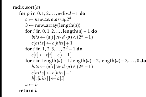
(In this code, the expression
![]() extracts the integer
whose binary representation is given by bits
extracts the integer
whose binary representation is given by bits
![]() of
of
![]() .)
An example of the steps of this algorithm is shown in Figure 11.8.
.)
An example of the steps of this algorithm is shown in Figure 11.8.
![\includegraphics[width=\textwidth ]{figs-python/radixsort}](img4447.png)
|
This remarkable algorithm sorts correctly because counting-sort is
a stable sorting algorithm. If
![]() are two elements of
are two elements of
![]() ,
and the most significant bit at which
,
and the most significant bit at which
![]() differs from
differs from
![]() has index
has index ![]() ,
then
,
then
![]() will be placed before
will be placed before
![]() during pass
during pass
![]() and subsequent passes will not change the relative order of
and subsequent passes will not change the relative order of
![]() and
and
![]() .
.
Radix-sort performs
![]() passes of counting-sort. Each pass requires
passes of counting-sort. Each pass requires
![]() time. Therefore, the performance of radix-sort is given
by the following theorem.
time. Therefore, the performance of radix-sort is given
by the following theorem.
If we think, instead, of the elements of the array being in the range
![]() , and take
, and take
![]() we obtain
the following version of Theorem 11.8.
we obtain
the following version of Theorem 11.8.
![\includegraphics[width=\textwidth ]{figs-python/countingsort}](img4391.png)